

Pruning is one of the oldest and most reliable ways to shrink a neural network: not every parameter contributes equally to a model’s predictions, so removing the least useful ones yields a smaller, cheaper model. Almost every pruning method, however, shares a single assumption - that the way to remove a parameter is to cut it out in one step. This post describes soft pruning, the method behind my IJCNN/WCCI 2024 paper, which instead decays unwanted parameters out of the network gradually while training continues. By giving the network time to redistribute the information held in those parameters before they disappear, soft pruning preserves accuracy at levels of sparsity where conventional “hard” pruning collapses to random guessing.
Hard Pruning and the Cost of a Sudden Cut
Any pruning method has to answer two separate questions: which parameters to remove, and how to remove them. The first question - selection - is well studied. Magnitude-based pruning ranks weights by their absolute value and removes the smallest, and remains popular precisely because it is simple and effective. More involved methods such as Optimal Brain Damage use second-order (Hessian) information to identify low-saliency parameters. Soft pruning is agnostic to this choice; the work focuses entirely on the second question.
It is the how that is almost always taken for granted. Whether a network is pruned in a single pass (one-shot), gradually over repeated prune-and-retrain cycles (iterative), or trained against a fixed sparsity mask, the parameter itself is removed suddenly - its value is set to zero in one step. The hypothesis behind soft pruning is that this sudden removal throws away the information stored in that parameter. At low sparsity this rarely matters, because enough capacity remains that retraining can relearn what was lost. At high sparsity it matters a great deal: there are too few parameters left to recover the discarded information, and accuracy falls off a cliff.
Soft Pruning: Decaying Weights Out
Rather than cutting a parameter out, soft pruning decays it smoothly towards zero over many batches while the rest of the network keeps training. The idea is that a parameter on its way out still holds useful information, and a gradual decay gives the surviving parameters time to absorb that information before it is gone.
The whole scheme collapses into a single modified update rule. Let W_{ij} be the parameter matrix, M_{ij} a pruning mask whose entries are 1 for parameters being pruned and 0 for those that remain, x \in (0, 1) a decay factor, and \Delta W_{ij} the gradient update:
For a parameter being pruned ( M_{ij} = 1 ) the second term vanishes and the weight is simply multiplied by x each step, decaying geometrically to zero while receiving no gradient. For a parameter that remains ( M_{ij} = 0 ) the first term vanishes and it trains as normal. Once the decay has run its course the masked weights are exactly zero and can be deleted for free, so there is no inference-time cost compared to hard pruning.
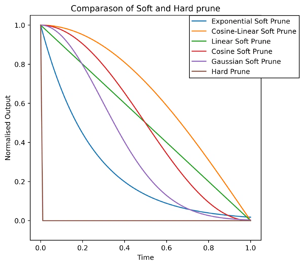
A number of decay schedules are possible - linear, cosine, Gaussian, exponential, and combinations of these. In practice they all converged to a similar end state on simple problems, and exponential decay reached it the fastest, so it is the schedule used throughout. One implementation detail is worth flagging: because magnitude-based selection assumes a weight’s size reflects its importance, it pairs poorly with the unbounded ReLU activation, where magnitude pruning behaves more like random pruning. Every network here therefore uses the bounded tanh activation.
What Soft Pruning Buys You
Soft pruning was evaluated on MNIST, FashionMNIST and CIFAR-10 across three tasks - classification, autoencoding and latent-space dimensionality reduction. The comparison is against both plain hard pruning and the stronger baseline of hard pruning followed by retraining. Crucially, soft pruning and the retraining baseline are given the same amount of training data, so any advantage comes from the method rather than extra compute.
Classification
On classification, soft pruning matches or beats hard pruning with retraining, and the gap widens sharply as sparsity increases. The headline result is on MNIST: a ten-way classifier retains over 60% accuracy with 97% of its parameters pruned, at a point where one-shot hard pruning has already collapsed to roughly 10% - no better than guessing.
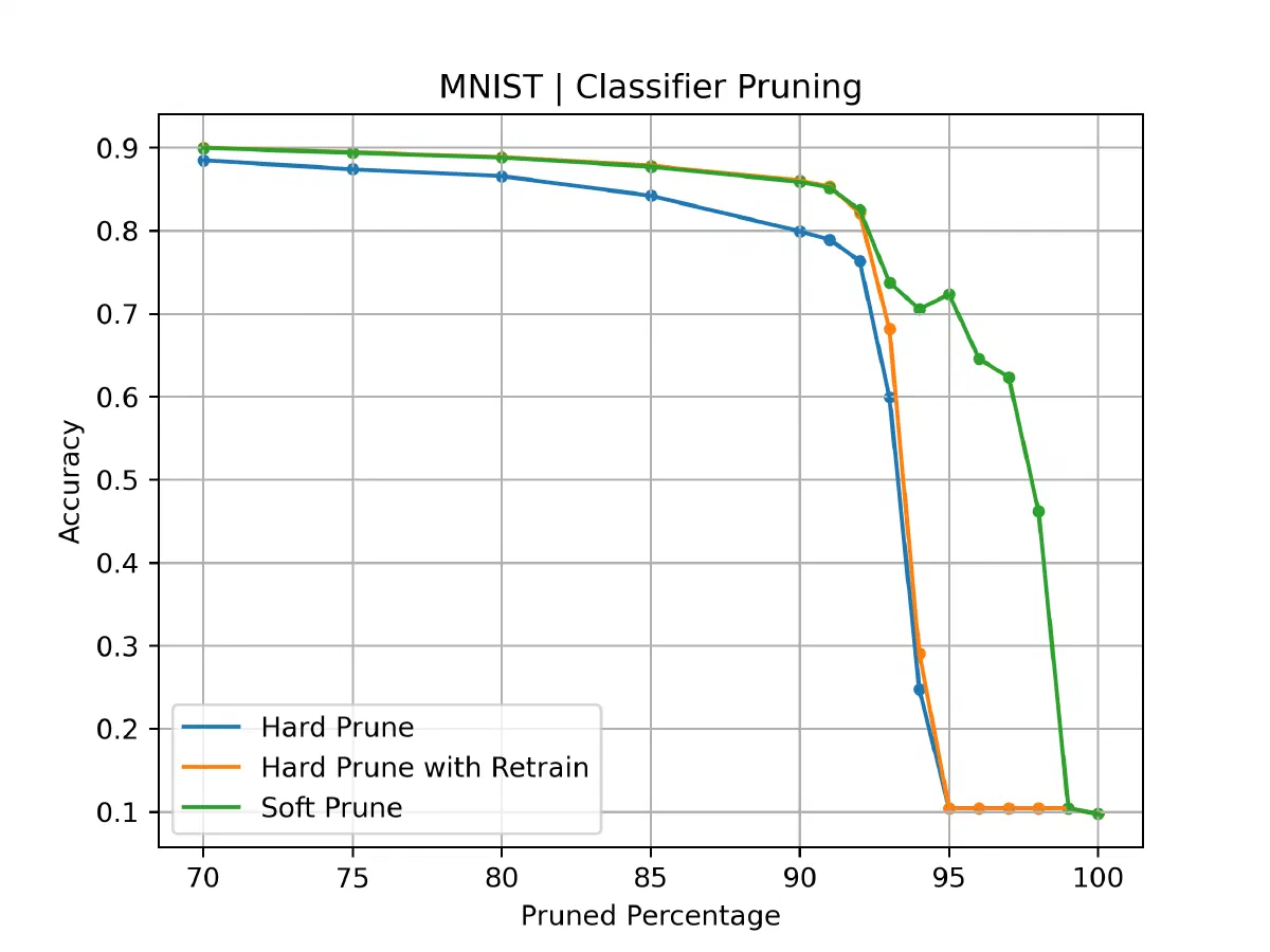
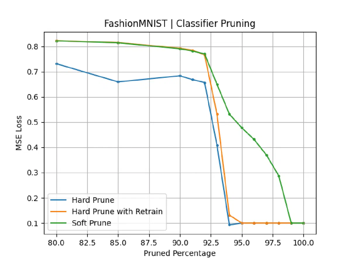
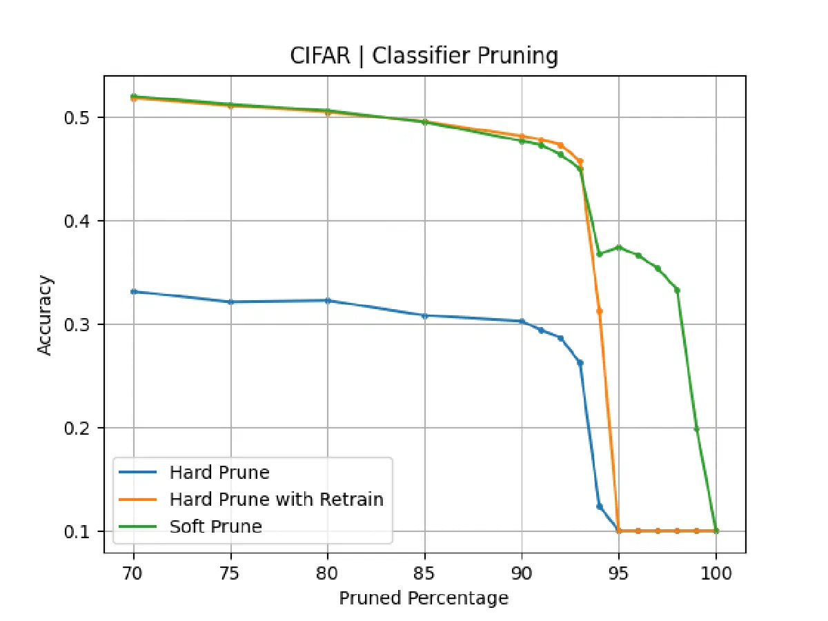
Table 1. Classification accuracy (%) at high pruning levels. Hard pruning - even with retraining - falls to random guessing once enough parameters are removed, whereas soft pruning degrades gracefully. The best result in each column is shown in bold.
| Dataset | Method | 90% | 95% | 97% |
|---|---|---|---|---|
| MNIST | Hard Prune | 79.9 | 10.4 | 10.4 |
| MNIST | Hard Prune & Retrain | 86.1 | 10.4 | 10.4 |
| MNIST | Soft Prune | 85.9 | 72.3 | 62.3 |
| FashionMNIST | Hard Prune | 68.4 | 10.0 | 10.0 |
| FashionMNIST | Hard Prune & Retrain | 79.3 | 10.0 | 10.0 |
| FashionMNIST | Soft Prune | 79.1 | 47.8 | 37.0 |
| CIFAR-10 | Hard Prune | 30.3 | 10.0 | 10.0 |
| CIFAR-10 | Hard Prune & Retrain | 48.1 | 10.0 | 10.0 |
| CIFAR-10 | Soft Prune | 47.7 | 37.4 | 35.4 |
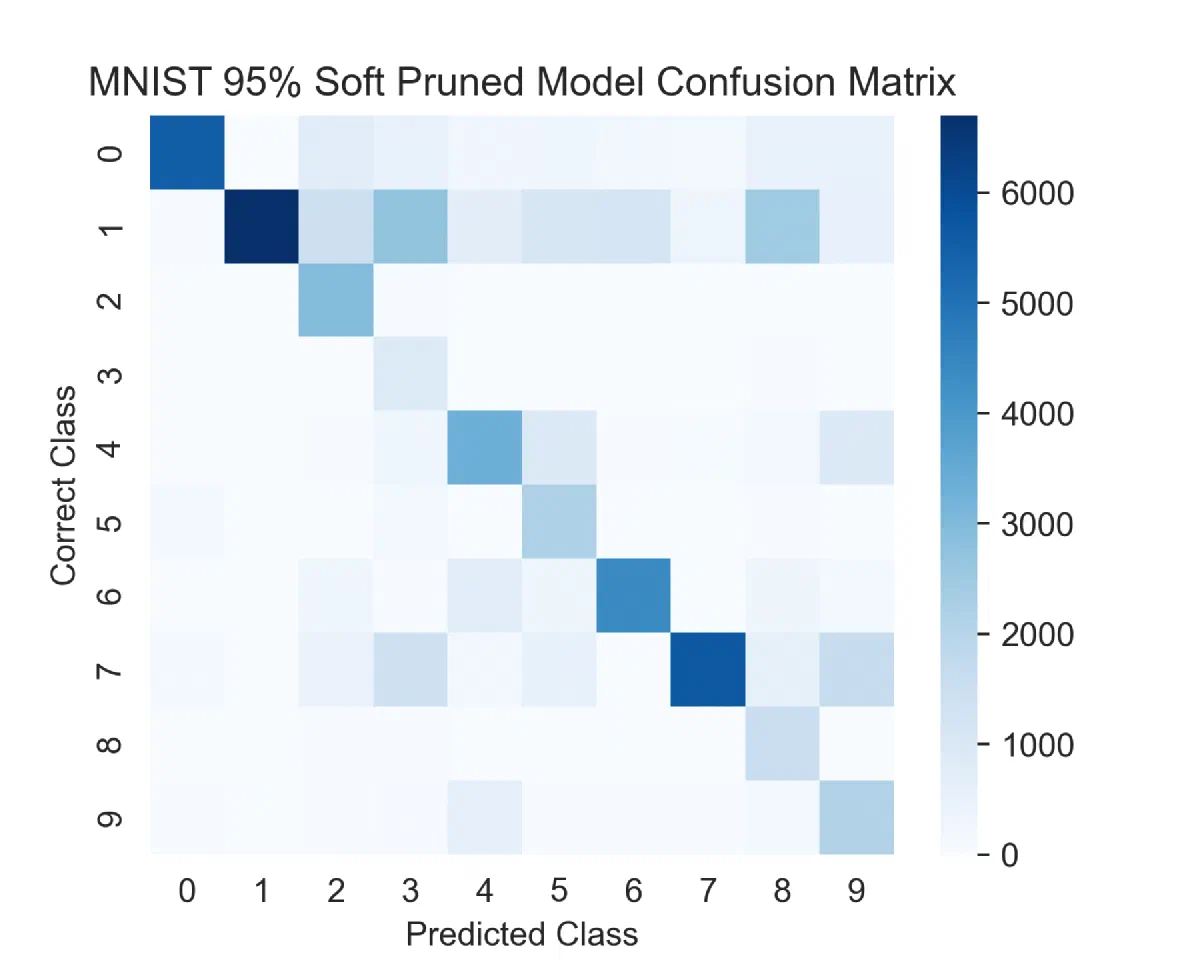
A recurring feature on the harder datasets is a plateau: on CIFAR-10, soft pruning levels off at around 35% accuracy once 70% or more of the network is pruned, well above random guessing, while hard pruning drops to the floor. This is consistent with the information-conservation hypothesis - soft pruning forces the features that carry the most accuracy to be compressed into the handful of nodes that remain, and only when even those cannot hold the features does accuracy finally break down. A confusion matrix of the 95%-pruned MNIST model bears this out: the classes that survive best are those with simpler, shared features, while the most distinctive classes are merged into them.
Autoencoding
The second task moves from labelling images to reconstructing them, pruning the decoder of a visual autoencoder. Here soft pruning again matches or outperforms hard pruning on reconstruction loss across every dataset, and the shape of the result echoes the classification experiments: up to around 90% pruning the two methods stay close, and the gap opens up once pruning becomes aggressive. Aggregated across the datasets, pruning between 80% and 90% gives a 0-13.1% improvement in loss, rising to as much as 17.6% at higher pruning levels.
The behaviour does vary by dataset. On MNIST the advantage is marginal until 90% pruned (0-1.4% lower loss), after which soft pruning pulls ahead by up to 9.2% before the loss of both methods begins to climb steeply. FashionMNIST is the clearest case - it is visually harder to reconstruct because each image carries more detail, and soft pruning preserves that detail for up to 16.7% lower loss as pruning increases. CIFAR follows MNIST’s shape, marginal (0-1.3%) up to 90% pruned and then up to 17% lower loss beyond it. Since the same parameters are ultimately removed in every case, the improvement points squarely to soft pruning preserving information that the sudden cut destroys.
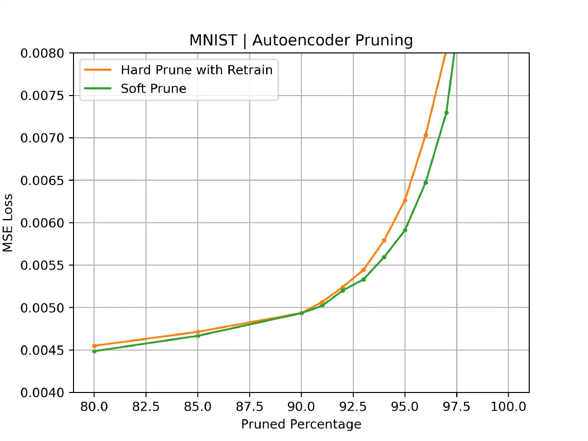
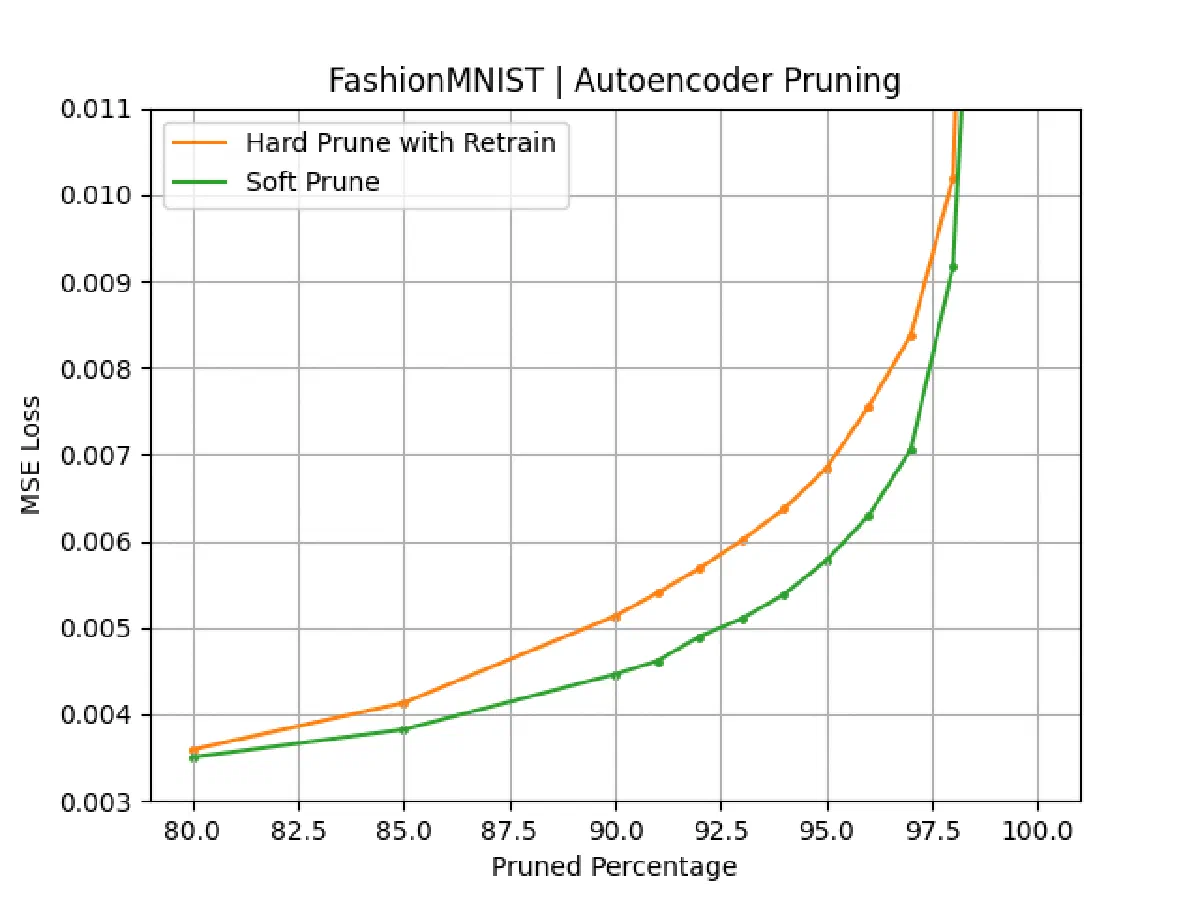
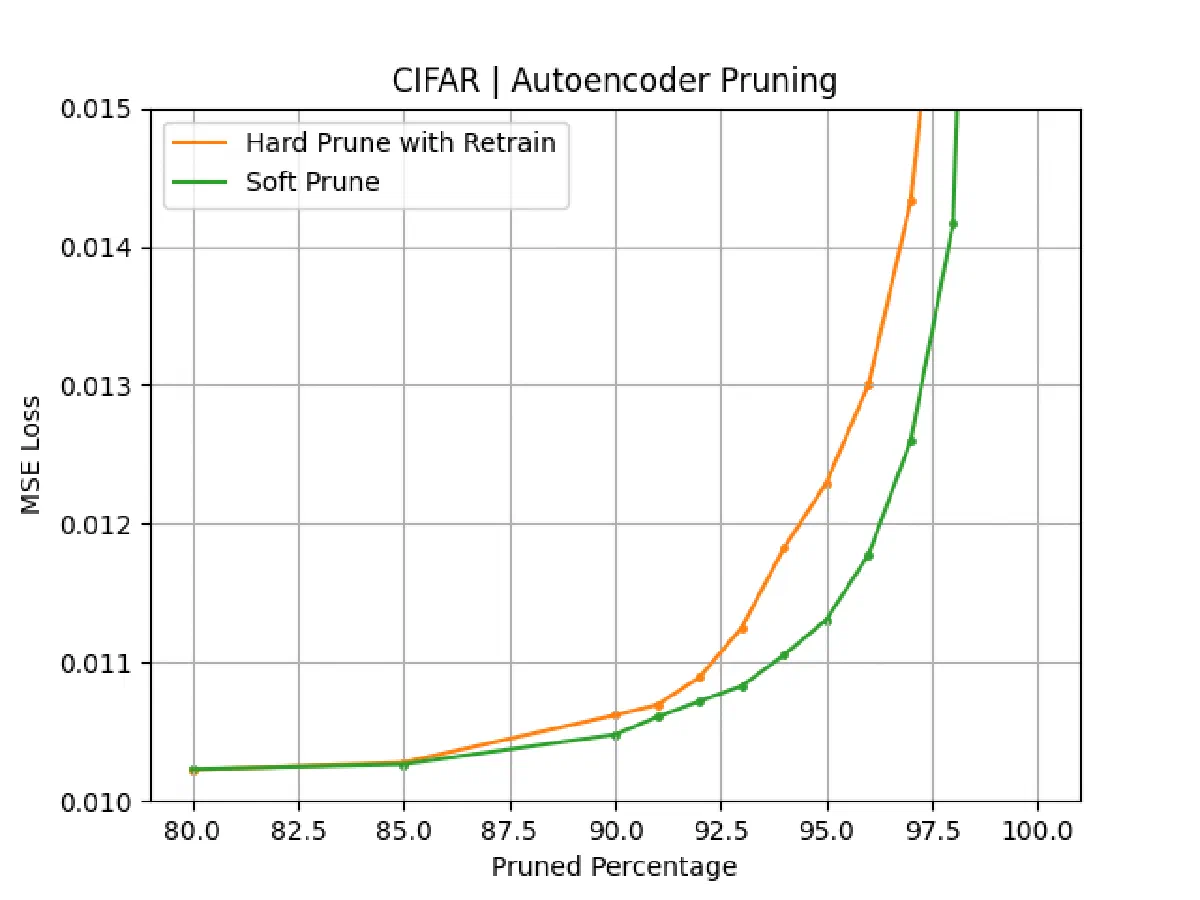
Table 2. Peak reduction in autoencoder reconstruction loss from soft pruning relative to hard pruning. Below roughly 90% pruning the two methods are within about 1.4% of each other on MNIST and CIFAR-10; the advantage shown here is reached as pruning becomes more aggressive.
| Dataset | Lower reconstruction loss vs hard pruning |
|---|---|
| MNIST | up to 9.2% |
| FashionMNIST | up to 16.7% |
| CIFAR-10 | up to 17% |
Latent Space Dimensionality Reduction
The third task is the most interesting: rather than thinning the weights, it shrinks the latent space itself by pruning whole nodes (and therefore whole latent dimensions), which keeps the representation small and cheaper to work with downstream.
To decide which nodes to remove, the method borrows skeletonization. A multiplicative gate m_i is attached to each node so that its value becomes n_i = a_i m_i , and the saliency of the node is measured as the gradient of the loss E with respect to that gate, s_i = \partial E / \partial a_i . A small saliency means the node has little effect on the loss and is safe to remove; the lowest-saliency nodes are pruned by decaying the weights on either side of them.
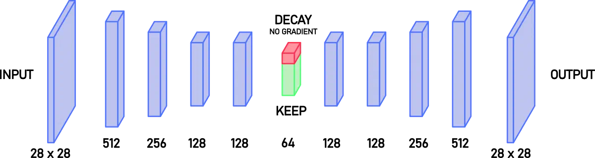
The gains here are the largest of the three tasks. Soft pruning beats hard pruning with retraining by a wide margin - up to 60.9% lower loss on MNIST, up to 35.8% on FashionMNIST, and over 10% on CIFAR (reaching 20.7% lower loss at 95% pruned). Just as telling, the loss stays close to that of the original unpruned model: on MNIST it rises by only 8.4% at 95% pruned, compared with a 154% increase for hard pruning with retraining.
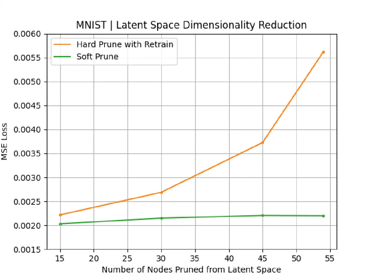
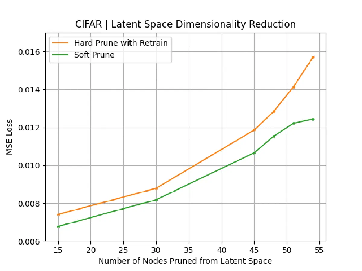
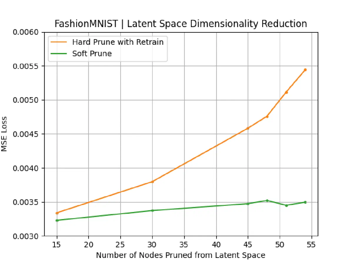
Table 3. Reconstruction loss (×10-3) when pruning latent-space dimensions, at 25%, 50% and 75% of the 64-node latent space removed. Soft pruning gives the lowest loss in every case; best results are shown in bold.
| Dataset | Method | 25% | 50% | 75% |
|---|---|---|---|---|
| MNIST | Hard Prune | 5.70 | 11.52 | 17.56 |
| MNIST | Hard Prune & Retrain | 2.21 | 2.69 | 3.73 |
| MNIST | Soft Prune | 2.02 | 2.15 | 2.20 |
| FashionMNIST | Hard Prune | 8.15 | 15.9 | 22.9 |
| FashionMNIST | Hard Prune & Retrain | 3.34 | 3.80 | 4.58 |
| FashionMNIST | Soft Prune | 3.23 | 3.37 | 3.47 |
| CIFAR | Hard Prune | 13.08 | 19.06 | 25.91 |
| CIFAR | Hard Prune & Retrain | 7.41 | 8.79 | 11.86 |
| CIFAR | Soft Prune | 6.77 | 8.18 | 10.66 |
Why It Works
The thread running through all three tasks is information conservation. A weight or node about to be removed still encodes something useful, and decaying it slowly while the rest of the network trains lets that information migrate into the parameters that survive. Hard pruning discards it in a single step, and at high sparsity there simply is not enough remaining capacity - nor, given a fixed retraining budget, enough data - to relearn it. That is why the advantage of soft pruning is small at low sparsity but grows steadily as more of the network is removed.
Looking Ahead
These results are established on feedforward dense layers, and the natural next step is to ask whether they carry over to convolutional, transformer and recurrent architectures, where the interactions between parameters are richer. There is also a more ambitious possibility hiding in the method: because soft pruning is a smooth, continuous optimisation rather than a discrete cut, it should be possible to optimise desired features into a latent space - or unwanted ones out - during pruning, leaving behind a compact representation that is fine-tuned for a particular task. Combined with quantisation, techniques like this continue to push genuinely capable models onto edge devices and into resource-constrained settings.
The full paper, Soft Pruning and Latent Space Dimensionality Reduction, is available here.