
Weight initialization is a necessary first step in all neural networks This work reviews the currently popular methods of weight initialization without using input data and proposes Constant Variance Weight Initialization. Applied to small neural networks, Constant Variance initialization is shown to result in an increase in training speed compared to Xavier initialization, a result which fails to generalize to larger neural networks. However, equivalent performance can be achieved on larger neural networks either by scaling the range of the S-shaped activation function or by reducing the standard deviation of the input and the standard deviation of the forward propagation. Constant Variance initialization is then compared to He initialization, where it shows no significant difference in training speed when applied to small neural networks, but results in an equal or improved training speed when applied to larger neural networks.
Constant Variance Weight Initialisation
Constant Variance weight initialization provides the neural network with an initial set of weights which ensure the propagated input has unit variance (and zero mean for symmetric activation functions) at each layer. This approach does not require knowledge of the input, beyond expecting it to have unit variance and zero mean, similar to Xavier and He initialization. To ensure a unit-variance input propagation, the weights of each layer are selected from a normal distribution whose standard deviation is a function of some coefficient determined by the activation function, chosen to re-normalize the input on each layer. This further ensures that the input of each layer is consistent, not shrinking nor growing exponentially through the network. Failing to ensure the input is consistently scaled across layers of the neural network can severely hamper neural network training.
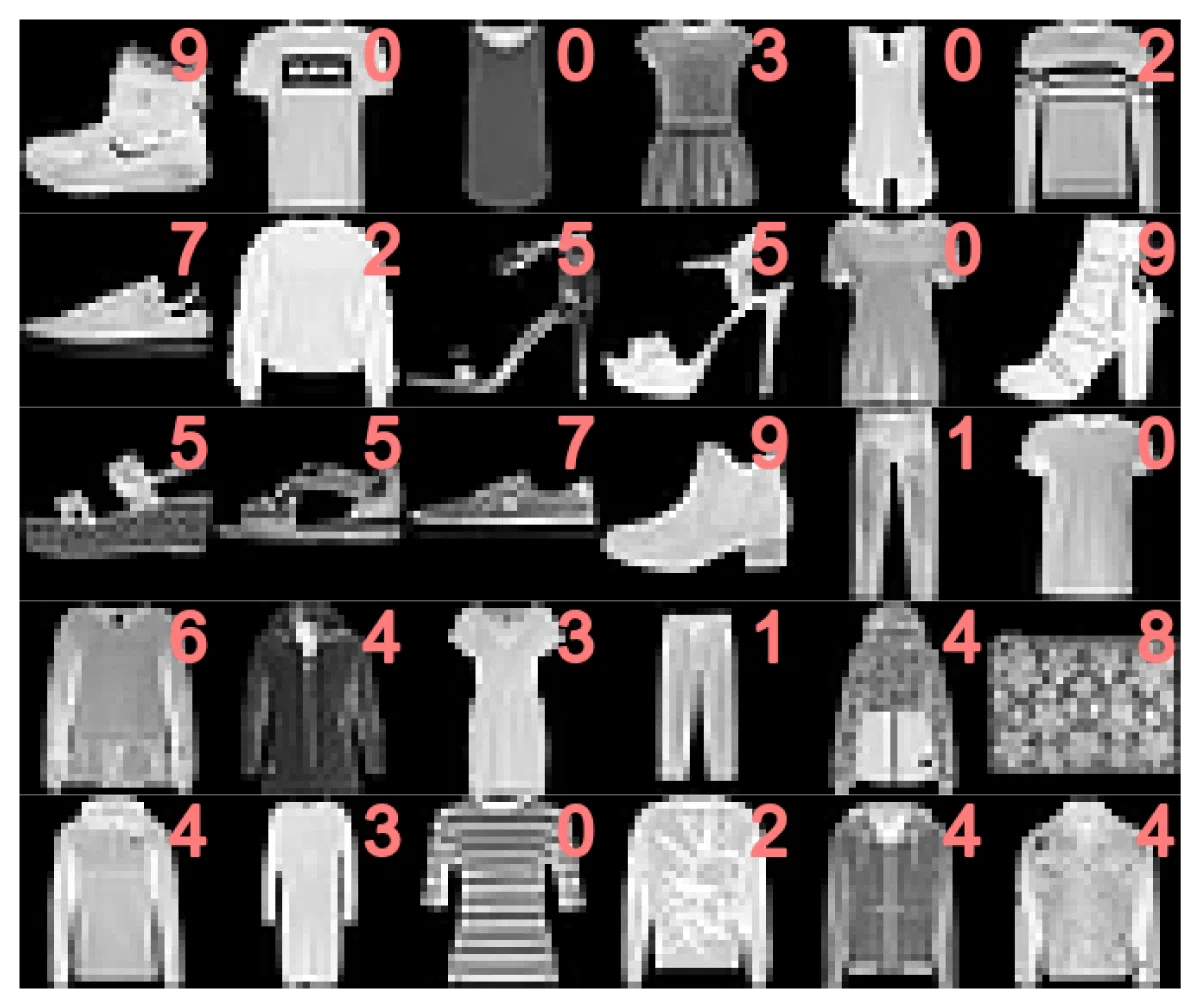
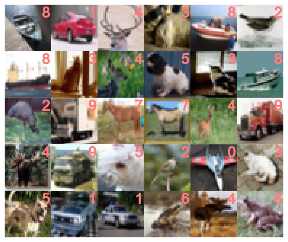
An empirical study was performed to identify the values which allow for the propagated input to maintain constant variance throughout each layer, following which these values were tested on the FashionMNIST [1] and CIFAR10 [2] datasets using different neural network architectures. A sample of each of these datasets is shown below. The standard deviation coefficients found empirically are given in Table 1.
To empirically find these coefficients, a two-layer neural network can be created with j nodes in each layer using activation function a . This can be given a random vector v , whose j elements are sampled from a standard normal distribution. The output o from this neural network, given the application of v , can be used to determine the scaling coefficient for activation function a : The coefficient is the value that scales the output to have unit standard deviation. This means the coefficient for activation a is simply
Due to the use of a random normal distribution as the input vector, this experiment must be repeated a number of times to reduce the statistical uncertainty of the coefficient.
Each of these coefficients could have equally been derived by calculation but the process is more involved. Consider there are n input weights to a node within a neural network, where each weight multiplied by its input provides an output which conforms to a standard normal distribution. Before the application of the activation function, the normal distributions are summed, resulting in an activation output distribution of
where a is the activation function and the sum of standard normal distributions is a different normal distribution of mean \mu_{new} and standard deviation of \sigma_{new} given by
Considering the output of the node after the application of the activation function does not generally have unit standard deviation, the coefficient of the standard deviation of the weights must convert the output distribution back to a standard normal distribution. Therefore, the weights must be initialized in the form of
where \mathcal{D} is some distribution with mean 0 and standard deviation c/\sqrt{n} . c is some coefficient which ensures a standard normal propagation given the activation function used. The \sqrt{n} term appears from the sum of the weights applied to the inputs, where it is assumed that each input is a standard normal distribution.
Therefore, the coefficient of the standard deviation is simply
For mathematically simple activation functions such as ReLU, this is a straightforward calculation, as provided by He et al. [3]. However, for even moderately complicated activation functions, this formula quickly becomes unwieldy, and although eventually the correct answer can be reached, it would be a significant burden on authors of new activation functions to perform such derivations. Furthermore, for certain activation functions, this is unsolvable without the use of a Taylor expansion or simplifying assumption (as used by Glorot and Bengio [4]), meaning at best only an approximation of the coefficient can be reached. Given current computational power, it is significantly easier, quicker and can be more accurate, to empirically derive the coefficients. The code for performing this and for running the experiments has been provided in the supplementary material and will be made open-source on paper publication.
Table 1. Scaling constants which maintain constant variance throughout each layer of a neural network for a given activation function. All coefficients were derived empirically using a two-layer neural network with a normal distribution as the input; the ReLU coefficient can additionally be derived theoretically, as given by He et al. The coefficients for the uniform distributions are given in terms of the bounds of the distribution rather than the standard deviation, for convenience.
| Activation Function | STD. Coefficient (Normal) | STD. Coefficient (Uniform) |
|---|---|---|
| Identity | 1.000 | ±1.732 |
| Logistic | 1.847 | ±3.198 |
| Tanh | 1.592 | ±2.758 |
| Softsign | 2.338 | ±4.049 |
| ReLU | 1.414 | ±2.449 |
| GELU | 1.534 | ±2.656 |
| ELU | 1.245 | ±2.180 |
| SiLU | 1.677 | ±2.904 |
| SELU | 1.000 | ±1.732 |
| Tanh8 | 1.015 | — |
| Tanh Half-Std | 1.200 | — |
Comparison to Xavier Initialization
Xavier Initialization is considered as a standard method to initialize neural networks that use S-shaped activation functions and would be expected to outperform Constant Variance initialization due to the latter causing the saturation of the nodes (where a standard normal distribution intersects with the extremities of the S-shaped function), reducing backward gradient flow and causing slower training. However, it is possible to resolve these issues by altering the range of the S-shape, or decreasing the standard deviation of the input and forward propagation such that it resides more within the near linear region of the S-shape.
FashionMNIST | Feedforward Network
Constant Variance weight initialization was compared to Xavier initialization on the Logistic Sigmoid, Tanh, Softsign, ReLU and ELU activation functions. The first experiment used the FashionMNIST [1] dataset on a feedforward neural network of architecture [28\times28, 100, 58, 38, 28, 10] . Similar to Xavier and He initialization, the biases were initialized to 0. To ensure a fair comparison, each experiment was run five times and the mean and standard deviation were plotted.
Constant Variance initialization was able to consistently outperform Xavier initialization on the S-shaped activation functions tested on training speed, performing significantly better on Softsign. Xavier initialization was also tested with ReLU and ELU, where Constant Variance initialization again either matched or beat its performance. Logistic Sigmoid was found to be an outlier on both initialization methods, taking significantly longer to train than the other activation functions. Constant Variance initialization likely performs poorly here because the mean is shifted on every layer up to 0.5, which the weight initialization then tries to push back to 0, causing excessive saturation. Unmitigated, this effect grows on each layer, resulting in poor forward propagation and reduced gradients in backpropagation.
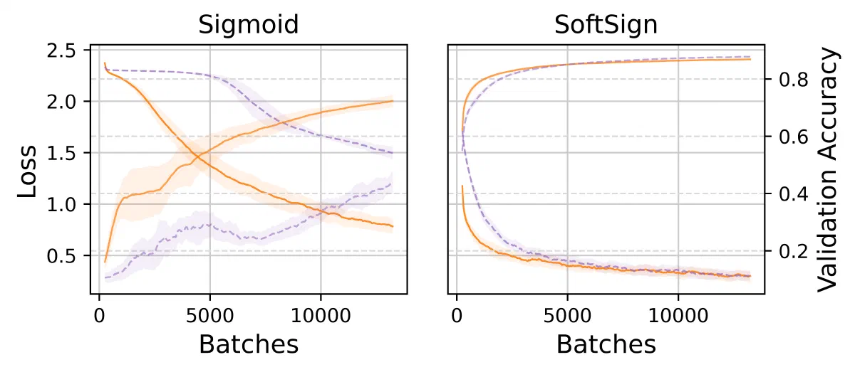
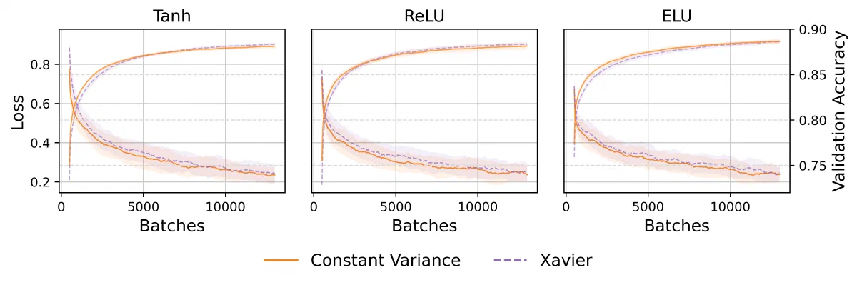
[28×28, 100, 58, 38, 28, 10] using either Xavier (purple dashed) or Constant Variance (orange solid) weight initialization. The mean and standard deviation of five repeated experiments are plotted.The averaged training loss is given in Table 2, where in almost every case Constant Variance initialization reaches a lower loss than Xavier initialization at the same batch number.
Table 2. The results shown in the figure above. In almost all cases, Constant Variance initialization is better than Xavier initialization. Values are the average of 100 data points centered on each batch number.
| Activation | Initialization | 2500 | 5000 | 7500 | 10000 | Final |
|---|---|---|---|---|---|---|
| Sigmoid | Xavier | 2.292 | 2.244 | 1.891 | 1.666 | 1.510 |
| Sigmoid | Const. Variance | 1.909 | 1.378 | 1.108 | 0.930 | 0.791 |
| Tanh | Xavier | 0.422 | 0.350 | 0.303 | 0.270 | 0.244 |
| Tanh | Const. Variance | 0.397 | 0.327 | 0.275 | 0.261 | 0.235 |
| ReLU | Xavier | 0.389 | 0.332 | 0.296 | 0.269 | 0.251 |
| ReLU | Const. Variance | 0.367 | 0.302 | 0.274 | 0.265 | 0.235 |
| Softsign | Xavier | 0.603 | 0.448 | 0.375 | 0.349 | 0.304 |
| Softsign | Const. Variance | 0.491 | 0.404 | 0.361 | 0.330 | 0.308 |
| ELU | Xavier | 0.380 | 0.334 | 0.296 | 0.279 | 0.246 |
| ELU | Const. Variance | 0.371 | 0.314 | 0.289 | 0.264 | 0.238 |
CIFAR10 | VGG19
To better understand the difference in the forward and backward propagation provided by the different methods of initialization, a deeper neural network of 32 layers with 1024 nodes in each layer was analyzed under different activation functions. The backpropagation of Constant Variance initialization was largest near the start of the network, whereas the backpropagation of Xavier initialization was largest nearer the end. It could be expected that a backpropagated gradient which is largest near the start of the network would train from the input, and so could allow a neural network using Constant Variance initialization to achieve faster training and higher performance, hence allowing a smaller network to train faster. Equally, the earlier layers may not need to be trained significantly, or in some cases at all [5], allowing Xavier initialization to achieve competitive performance.
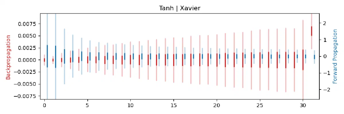
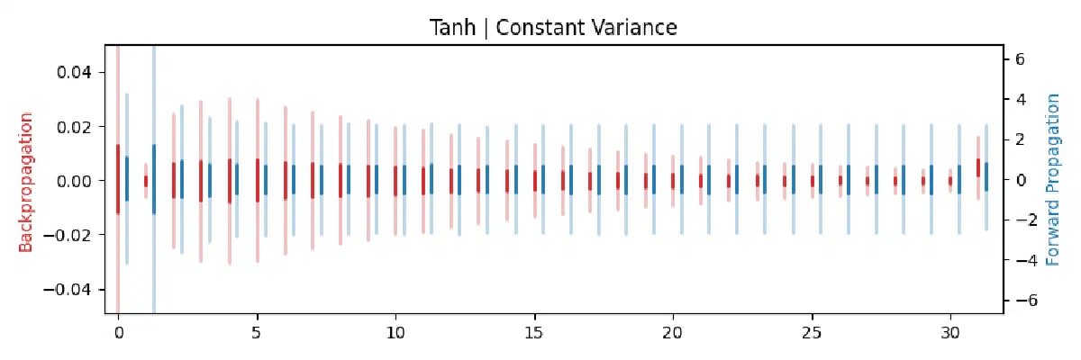
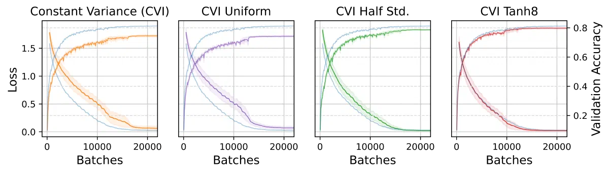
The next experiment analyzed the difference between Xavier and Constant Variance initialization when applied to a 19-layer VGG-inspired [6] network adapted for CIFAR10 [2]. This showed more promising results for ReLU-shaped activation functions: Xavier initialization was found to stall at the beginning of training whereas Constant Variance initialization does not. However, when applying Constant Variance initialization with the Tanh activation function, it was found to perform significantly worse than Xavier initialization, requiring a significantly longer training time and achieving a lower final accuracy.
A graph of the forward propagation was plotted to better understand the reason for this. From analyzing the forward propagation, it appears many of the nodes are saturating when constant variance is used: the application of the weights increases the standard deviation, then the application of Tanh decreases it, saturating nodes whose values lie on the extremities of the standard normal. This process is present throughout the neural network. When the nodes become saturated, the training time can increase due to the reduced gradient reaching those nodes, preventing them from training as quickly as non-saturated nodes.
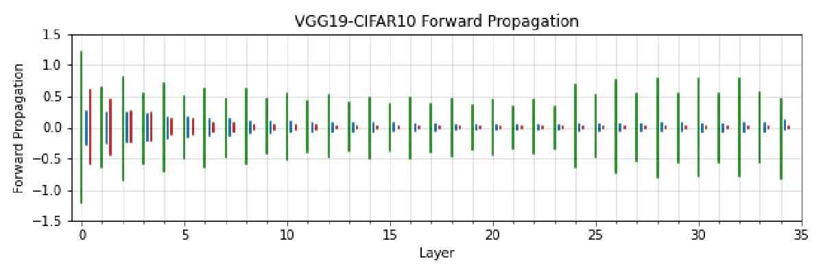
A further test was used to determine whether, rather than needing to consider backpropagation as is done in Xavier initialization, it would be sufficient to simply initialize the weights to ensure a forward propagation within the linear region of the S-shaped activation function. This was first tested by renormalizing the input to have half-standard deviation, then initializing the weights to ensure a half-standard deviation forward propagation. Doing so ensured that the forward propagation was largely contained within the linear region of Tanh; the training is initially slower but converges to that found when using Xavier initialization over the course of training, suggesting that this is a plausible explanation.
This was additionally tested by keeping the input normalized, but scaling the range of the Tanh activation function to have a larger linear region (Tanh8). This again worked significantly better than standard Constant Variance initialization and achieved a performance equal to Xavier initialization in loss, and only slightly lower in accuracy. Notably, the forward propagation using this method appears to be more similar to the forward propagation found when using Xavier initialization. This suggests that the saturation of the nodes caused by Constant Variance initialization was the reason the network trained slower than when Xavier initialization was used.
Comparison to He Initialization
He initialization was derived as a method of constant variance initialization for ReLU specifically, so it is the natural baseline to compare against for ReLU-shaped activation functions. Whereas the comparison to Xavier focused on S-shaped functions, here the focus is on the ReLU-shaped family - ReLU, ELU, GELU, SiLU and SELU.
FashionMNIST | Feedforward Network
Constant Variance initialization was compared to He initialization on the ReLU-shaped activation functions. Again, both methods were compared on a feedforward neural network which used the same architecture and optimization procedure as before, trained on the FashionMNIST dataset. No significant differences between the initialization methods were observed. SiLU and GELU performed negligibly better on loss with Constant Variance initialization, and SELU performed negligibly better on loss with He initialization. It is assumed that this is because there are too few layers - too little complexity - for any significant difference to present itself.
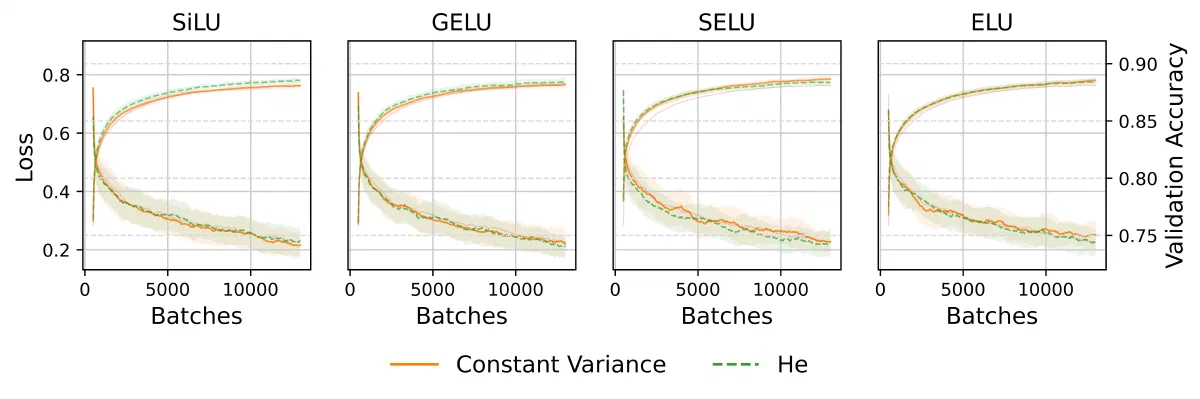
[28×28, 100, 58, 38, 28, 10] trained on FashionMNIST, initialized using either He (green dashed) or Constant Variance (orange solid) weight initialization for a range of ReLU-shaped activation functions.CIFAR10 | VGG19
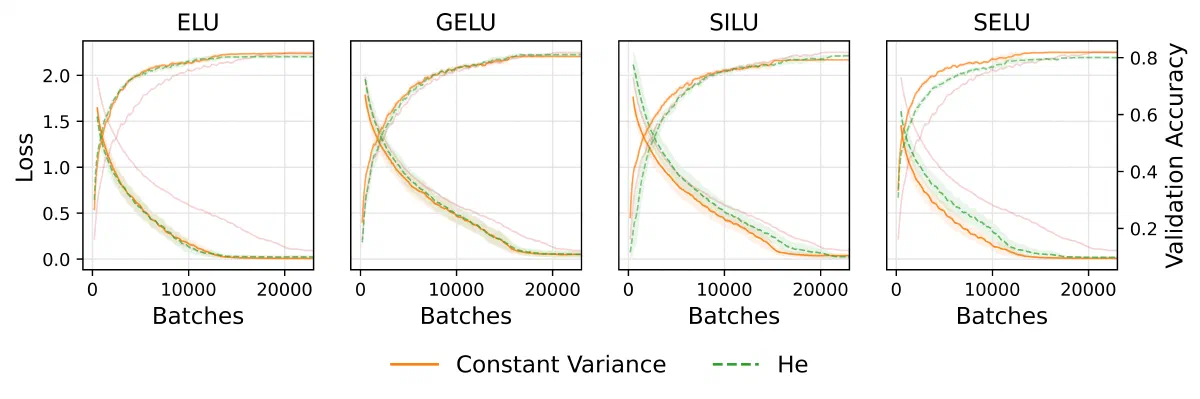
Constant Variance initialization was then compared to He initialization on the same 19-layer VGG-inspired neural network, using the same optimization procedure as before, trained to classify the CIFAR10 dataset. Here, Constant Variance initialization was able to achieve an improvement in accuracy for the ELU and SELU activation functions compared to He initialization, and was able to approximately match or increase the training speed on every activation function used. Additionally, Constant Variance initialization was consistently able to achieve a lower loss throughout training for both SiLU and SELU, and was able to match the performance of He initialization for GELU and ELU.
Every activation function using the correct initialization coefficient was able to consistently outperform ReLU, which suggests that modern neural networks should potentially look towards alternative ReLU-shaped activation functions - which allow negative values to train - to achieve faster training and lower loss upon convergence.
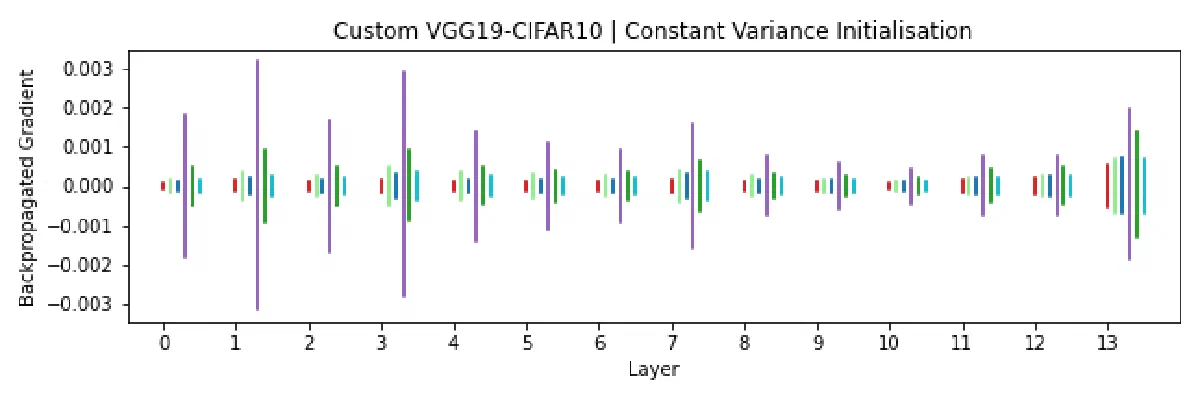
To analyze the difference in the forward and backward propagation between He initialization and Constant Variance initialization, the back-propagated gradient over the convolutional layers of the custom VGG19 neural network was plotted for each activation function. This illustrates that the gradients provided by Constant Variance initialization are, in this instance, generally equal to or greater than those provided by He initialization, which would account for the increased training speed provided by Constant Variance initialization. The gradient provided by SELU in particular is far greater when using He initialization compared to using Constant Variance initialization, yet SELU has a slower training speed when used with He initialization.
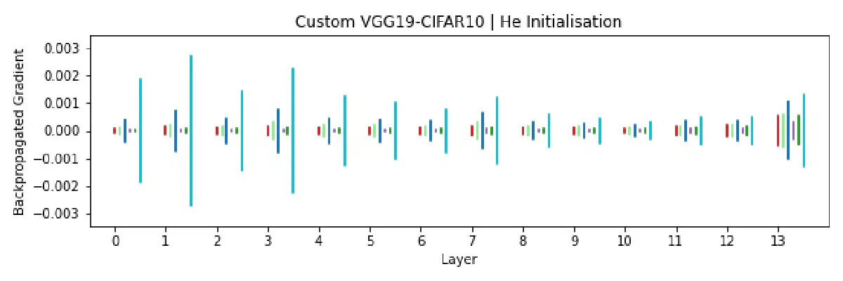
The averaged training loss across both datasets is given in Table 3.
FashionMNIST
Table 3 (FashionMNIST). The results shown in the He versus Constant Variance figures above. Values are the average of 100 data points centered on each batch number.
| Activation | Initialization | 2500 | 5000 | 7500 | 10000 | Final |
|---|---|---|---|---|---|---|
| ELU | He | 0.424 | 0.372 | 0.326 | 0.311 | 0.263 |
| ELU | Const. Variance | 0.427 | 0.350 | 0.332 | 0.318 | 0.270 |
| GELU | He | 0.419 | 0.358 | 0.331 | 0.309 | 0.245 |
| GELU | Const. Variance | 0.427 | 0.356 | 0.335 | 0.303 | 0.243 |
| SiLU | He | 0.422 | 0.361 | 0.332 | 0.316 | 0.257 |
| SiLU | Const. Variance | 0.426 | 0.362 | 0.331 | 0.306 | 0.258 |
| SELU | He | 0.411 | 0.347 | 0.310 | 0.306 | 0.234 |
| SELU | Const. Variance | 0.430 | 0.366 | 0.345 | 0.297 | 0.261 |
CIFAR10
Table 3 (CIFAR10). The results shown in the He versus Constant Variance figures above. Values are the average of 100 data points centered on each batch number.
| Activation | Initialization | 5000 | 10000 | 15000 | 20000 | Final |
|---|---|---|---|---|---|---|
| ELU | He | 0.534 | 0.138 | 0.026 | 0.021 | 0.024 |
| ELU | Const. Variance | 0.565 | 0.201 | 0.014 | 0.007 | 0.006 |
| GELU | He | 0.871 | 0.502 | 0.191 | 0.054 | 0.055 |
| GELU | Const. Variance | 0.845 | 0.445 | 0.191 | 0.060 | 0.056 |
| SiLU | He | 0.879 | 0.478 | 0.265 | 0.089 | 0.016 |
| SiLU | Const. Variance | 0.857 | 0.413 | 0.140 | 0.031 | 0.034 |
| SELU | He | 0.623 | 0.343 | 0.081 | 0.019 | 0.022 |
| SELU | Const. Variance | 0.445 | 0.131 | 0.016 | 0.008 | 0.008 |
Conclusion
When applied to small neural networks using S-shaped activation functions on visual classification tasks, Constant Variance initialization was found to result in faster training than Xavier initialization. This does not generalize well to larger neural networks due to the saturation of the nodes. Mitigating for this, by either decreasing the standard deviation of the input (and forward propagation) or increasing the range of the activation function, Constant Variance initialization performs almost equivalently to Xavier initialization - without needing to know the number of nodes in the succeeding layer.
Small neural networks using ReLU-shaped activation functions do not present significant differences in training speed when applying either Constant Variance initialization or He initialization on visual classification tasks. Larger neural networks were found to consistently train at a similar or faster speed when using Constant Variance initialization compared to using He initialization, while achieving a similar final loss and accuracy on the problems tested. Taken together, Constant Variance initialization offers a single, empirically-derived recipe that extends the constant-variance guarantee of He initialization to any activation function, without the per-function derivations such a guarantee would otherwise require.
References
- Han Xiao, Kashif Rasul, and Roland Vollgraf. Fashion-MNIST: a novel image dataset for benchmarking machine learning algorithms. 2017.
- Alex Krizhevsky. Learning multiple layers of features from tiny images. Master’s thesis, University of Toronto, 2009.
- Kaiming He, Xiangyu Zhang, Shaoqing Ren, and Jian Sun. Delving deep into rectifiers: Surpassing human-level performance on ImageNet classification. In 2015 IEEE International Conference on Computer Vision (ICCV), pages 1026–1034, 2015.
- Xavier Glorot and Yoshua Bengio. Understanding the difficulty of training deep feedforward neural networks. In Proceedings of the Thirteenth International Conference on Artificial Intelligence and Statistics (AISTATS), pages 249–256, 2010.
- Weipeng Cao, Xizhao Wang, Zhong Ming, and Jinzhu Gao. A review on neural networks with random weights. Neurocomputing, 275:278–287, 2018.
- Karen Simonyan and Andrew Zisserman. Very deep convolutional networks for large-scale image recognition. In International Conference on Learning Representations (ICLR), 2015.